Mean Value Theorem Calculator

Mean Value Theorem Calculator

Discover the point(s) where a function's average rate of change equals its instantaneous rate of change with our intuitive Mean Value Theorem Calculator. 

It will generate a comprehensive step-by-step solution, helping you understand the core principles of the Mean Value Theorem in a practical and straightforward manner.

What is the mean value theorem?

The Mean Value Theorem is a fundamental principle in calculus. It states:  

“For any smooth and continuous function over a specific range [a, b], there must be at least one point within that range where the function's instantaneous rate of change is equal to its average rate of change.”

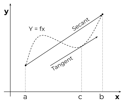
In other words, it guarantees that within the given interval, there exists a point where the slope of the tangent to the function's curve is the same as the slope of the secant line connecting the endpoints of the interval.

Understanding with an example:

Imagine you're going on a road trip between two cities, City A and City B. You drive at different speeds throughout the trip, and you want to find out if there was a moment when your speed was equal to your average speed for the entire journey.

The Mean Value Theorem is like a rule that says: If you drove smoothly and didn't make any sudden, jerky movements (like instantly changing your speed), then there must have been at least one moment during your trip when your speed exactly matched your average speed for the entire journey.

In more general terms, the MVT says that if a curve is smooth and doesn't have any abrupt changes, then at least at one point on the curve, the slope (or steepness) of the curve will match the average slope of the curve over a certain range.

Formula of mean value theorem:

Mathematically, it can be expressed as:

f'(c) = (f(b) - f(a)) / (b - a)

where c is a point in the interval (a, b), f'(c) is the derivative of the function f(x) at the point c, and (f(b) - f(a)) / (b - a) is the average rate of change of the function over the interval [a, b].

How to calculate the mean value theorem?

1. Verify the function is continuous on [a, b] and differentiable on (a, b).
2. Calculate the average rate of change of the function over the interval [a, b] using the formula: (f(b) - f(a)) / (b - a).
3. Find the derivative of the function, f'(x).
4. Solve the equation f'(x) = (f(b) - f(a)) / (b - a) for x to find the point(s).

Example 1:

Let's consider the function f(x) = x² on the interval [1, 3]. We'll apply the Mean Value Theorem to find the point where the function's instantaneous rate of change is equal to its average rate of change.

The average rate of change:

(f(3) - f(1)) / (3 - 1) = (9 - 1) / (3 - 1) = 8 / 2 = 4

Derivative of the function (instantaneous rate of change):

f'(x) = 2x (applying power rule)

Equate the average rate of change to the derivative:

2x = 4

Solve for x:

x = 4 / 2 = 2

So, there exists a point, x = 2, where the instantaneous rate of change is equal to the average rate of change. This point is (2, f(2)) = (2, 4).

Example 2:

Take the function g(x) = x³ - 3x² + 2x on the interval [-1, 2]. 

The average rate of change:

(g(2) - g(-1)) / (2 - (-1)) = (8 - 12 + 4 - (-1 - 3 + 2)) / 3 = (0 + 1) / 3 = 1 / 3

Derivative of the function (instantaneous rate of change):

g'(x) = 3x² - 6x + 2

Equate the average rate of change to the derivative:

3x² - 6x + 2 = 1 / 3

Solve for x:

3x² - 6x + 2 - 1/3 = 0

9x² - 18x + 6 - 1 = 0

9x² - 18x + 5 = 0

Using the quadratic formula, we find two solutions: x ≈ 0.276 and x ≈ 1.724.

So, there are two points within the interval [-1, 2] where the instantaneous rate of change is equal to the average rate of change. These points are approximately (0.276, g(0.276)) and (1.724, g(1.724)).

Real-Life applications:

• Analyzing velocity and acceleration: In physics, the MVT can help determine the relationship between a moving object's velocity and acceleration over time, as well as locate points where the instantaneous velocity equals the average velocity.
• Understanding growth rates: In biology and economics, the MVT can be used to analyze the growth rates of populations, investments, or other quantities that change over time.
• Designing efficient transportation routes: In transportation planning, the MVT can be used to find the optimal route between two points, taking into account factors like speed limits and traffic conditions.
• Predicting behavior in systems: In engineering and computer science, the MVT can be applied to analyze the behavior of complex systems and predict how changes in one part of the system will affect the system as a whole.